Detailed walk-through of de novo CIDER (dnCIDER) on pancreas data
Source:vignettes/dnCIDER.Rmd
dnCIDER.RmdIntroduction
This vignette performs dnCIDER on a cross-species pancreas dataset. It is aimed to show the underneath structure of dnCIDER compared to the other high-level vignette (see Getting Start with De Novo CIDER (dnCIDER): Cross-Species Pancreas Integration).
Set up
In addition to CIDER, we will load the following packages:
library(CIDER)
library(Seurat)
#> Loading required package: SeuratObject
#> Loading required package: sp
#> 'SeuratObject' was built under R 4.4.0 but the current version is
#> 4.4.1; it is recomended that you reinstall 'SeuratObject' as the ABI
#> for R may have changed
#>
#> Attaching package: 'SeuratObject'
#> The following objects are masked from 'package:base':
#>
#>     intersect, t
library(parallel)
library(cowplot)
Load example data
The example data can be downloaded from https://figshare.com/s/d5474749ca8c711cc205.
Pancreatic cell data contain cells from human (8241 cells) and mouse (1886 cells).
# Download the data
data_url <- "https://figshare.com/ndownloader/files/31469387"
data_file <- file.path(tempdir(), "pancreas_counts.RData")

if (!file.exists(data_file)) {
  message("Downloading data...")
  download.file(data_url, destfile = data_file, mode = "wb")
}
#> Downloading data...
data_env <- new.env()
loaded_objects <- load(file = data_file, envir = data_env)
pancreas_counts <- data_env[[loaded_objects[1]]]
load("../data/pancreas_meta.RData") # meta data/cell information
seu <- CreateSeuratObject(counts = pancreas_counts, meta.data = pancreas_meta)
table(seu$Batch)
#>
#> human mouse
#>  8241  1886
Perform initial clustering
seu_list <- Seurat::SplitObject(seu, split.by = "Batch")
seu_list <- mclapply(seu_list, function(x) {
  x <- NormalizeData(x, normalization.method = "LogNormalize",
                     scale.factor = 10000, verbose = FALSE)
  x <- FindVariableFeatures(x, selection.method = "vst",
                            nfeatures = 2000, verbose = FALSE)
  x <- ScaleData(x, verbose = FALSE, vars.to.regress = "Sample")
  x <- RunPCA(x, features = VariableFeatures(object = x), verbose = FALSE)
  x <- FindNeighbors(x, dims = 1:15, verbose = FALSE)
  x <- FindClusters(x, resolution = 0.6, verbose = FALSE)
  return(x)
})| 0 | 1 | 2 | 3 | 4 | 5 | 6 | 7 | 8 | 9 | 10 | 11 | 12 | 13 | 14 | 15 | 16 | 17 | 18 | |
|---|---|---|---|---|---|---|---|---|---|---|---|---|---|---|---|---|---|---|---|
| acinar | 0 | 0 | 823 | 0 | 0 | 0 | 1 | 1 | 2 | 102 | 0 | 0 | 0 | 0 | 0 | 0 | 0 | 3 | 0 |
| activated_stellate | 0 | 0 | 0 | 1 | 0 | 0 | 0 | 0 | 269 | 0 | 0 | 0 | 0 | 0 | 0 | 0 | 1 | 4 | 0 |
| alpha | 1067 | 3 | 0 | 0 | 0 | 665 | 0 | 0 | 0 | 0 | 251 | 243 | 1 | 6 | 0 | 0 | 1 | 0 | 4 |
| b_cell | 0 | 0 | 0 | 0 | 0 | 0 | 0 | 0 | 0 | 0 | 0 | 0 | 0 | 0 | 0 | 0 | 0 | 0 | 0 |
| beta | 1 | 886 | 2 | 812 | 740 | 1 | 0 | 0 | 0 | 0 | 2 | 0 | 3 | 2 | 1 | 0 | 4 | 0 | 1 |
| delta | 0 | 3 | 2 | 1 | 3 | 0 | 0 | 0 | 0 | 0 | 1 | 0 | 215 | 1 | 216 | 0 | 148 | 0 | 2 |
| ductal | 1 | 1 | 6 | 0 | 0 | 0 | 469 | 386 | 0 | 169 | 0 | 0 | 1 | 0 | 0 | 0 | 0 | 0 | 0 |
| endothelial | 0 | 0 | 0 | 0 | 0 | 0 | 0 | 0 | 1 | 0 | 0 | 0 | 0 | 0 | 0 | 212 | 0 | 1 | 0 |
| epsilon | 0 | 0 | 0 | 0 | 0 | 0 | 0 | 0 | 0 | 0 | 0 | 0 | 8 | 8 | 0 | 0 | 1 | 0 | 0 |
| gamma | 1 | 1 | 0 | 0 | 0 | 0 | 0 | 0 | 0 | 0 | 1 | 0 | 3 | 210 | 0 | 0 | 25 | 0 | 0 |
| immune_other | 0 | 0 | 0 | 0 | 0 | 0 | 0 | 0 | 0 | 0 | 0 | 0 | 0 | 0 | 0 | 0 | 0 | 0 | 0 |
| macrophage | 0 | 0 | 0 | 0 | 0 | 0 | 0 | 0 | 0 | 0 | 0 | 0 | 0 | 0 | 0 | 0 | 0 | 0 | 39 |
| mast | 0 | 0 | 0 | 0 | 0 | 0 | 0 | 0 | 0 | 0 | 0 | 0 | 0 | 0 | 0 | 0 | 0 | 0 | 25 |
| quiescent_stellate | 1 | 0 | 0 | 1 | 0 | 0 | 1 | 0 | 4 | 0 | 0 | 0 | 0 | 0 | 0 | 0 | 0 | 153 | 0 |
| schwann | 0 | 0 | 0 | 0 | 0 | 0 | 0 | 0 | 10 | 0 | 0 | 0 | 0 | 0 | 0 | 0 | 0 | 0 | 0 |
| t_cell | 0 | 0 | 0 | 0 | 0 | 0 | 0 | 0 | 0 | 0 | 0 | 0 | 0 | 0 | 0 | 0 | 0 | 0 | 7 |
seu_list <- mclapply(seu_list, RunTSNE, dims = 1:15)
p1 <- scatterPlot(seu_list[[1]], "tsne", colour.by = "seurat_clusters")
p2 <- scatterPlot(seu_list[[2]], "tsne", colour.by = "seurat_clusters")
cowplot::plot_grid(p1,p2)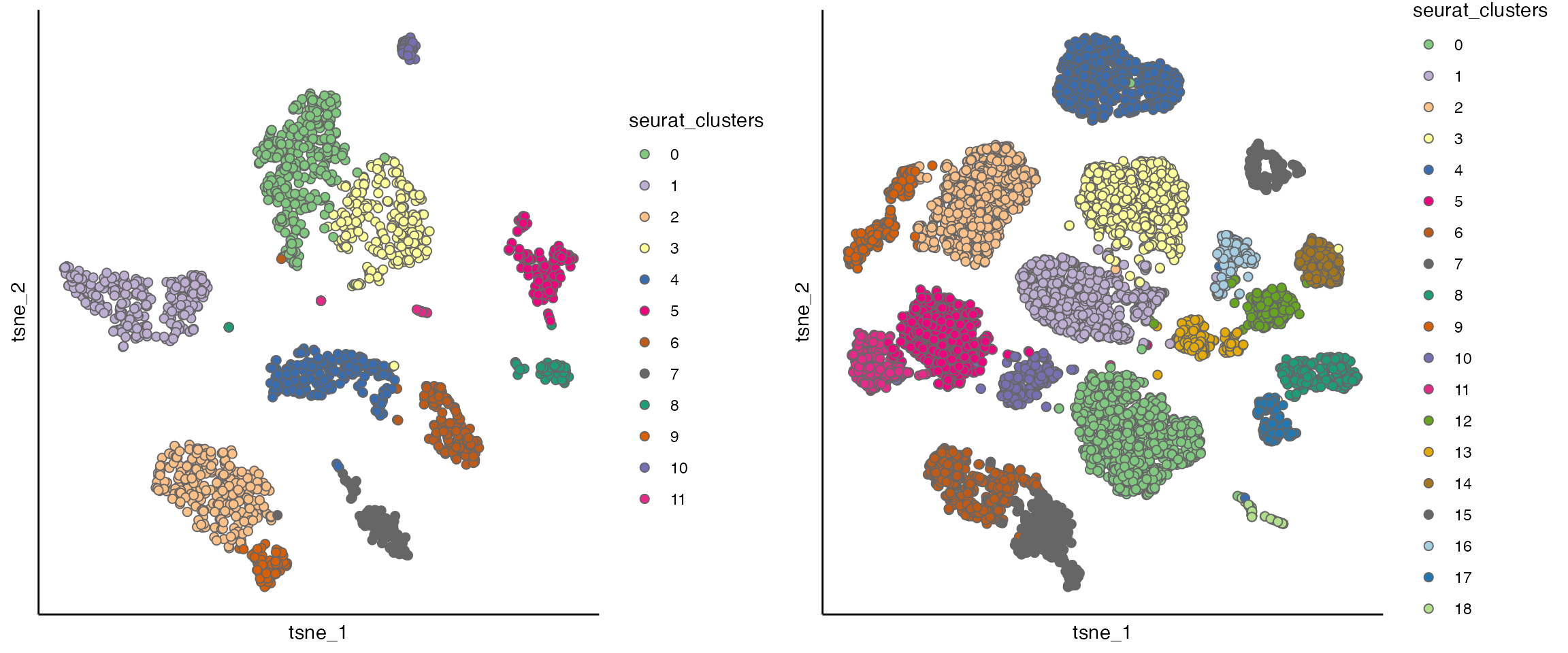
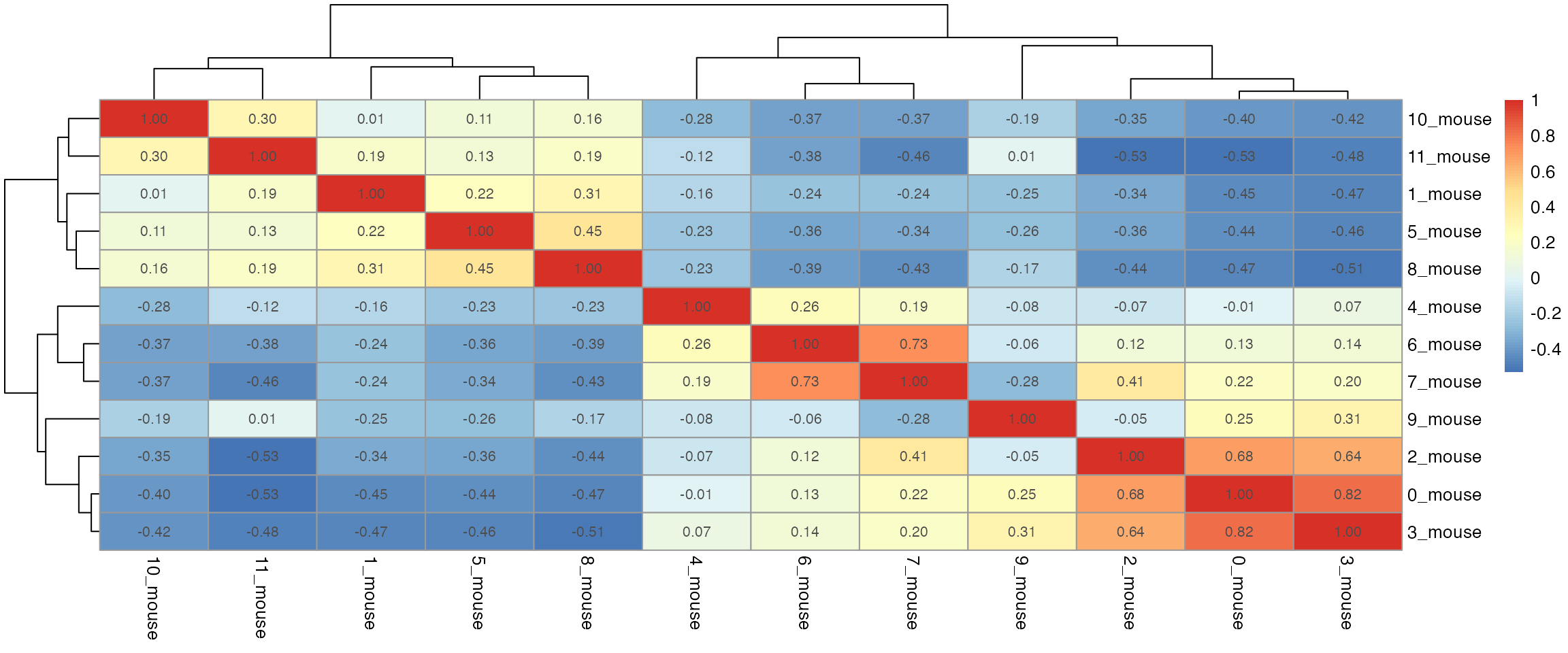
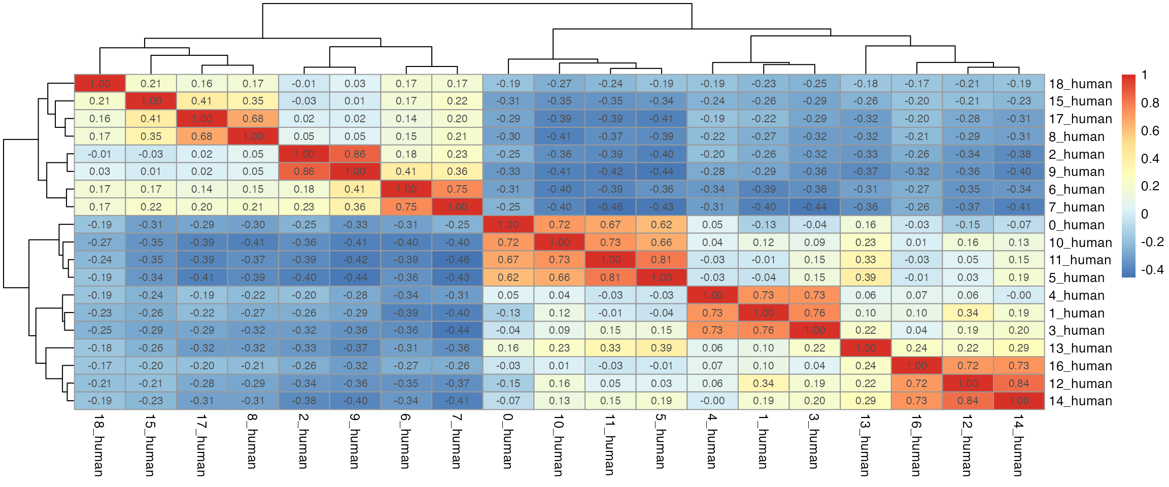
dist_coef <- getDistMat(seu_list, downsampling.size = 50)
#>   |                                                                              |                                                                      |   0%  |                                                                              |===================================                                   |  50%  |                                                                              |======================================================================| 100%
par(mfrow = c(length(seu_list),1))
for(i in which(sapply(dist_coef, function(x) return(!is.null(x))))){
  tmp <- dist_coef[[i]] + t(dist_coef[[i]])
  diag(tmp) <- 1
  pheatmap::pheatmap(tmp, display_numbers = TRUE)
}
for(seu_itor in 1:2){
  tmp <- dist_coef[[seu_itor]] + t(dist_coef[[seu_itor]])
  diag(tmp) <- 1
  tmp <- 1 - tmp
  hc <- hclust(as.dist(tmp), method = "average")
  hres <- cutree(hc, h = 0.4)
  df_hres <- data.frame(hres)
  df_hres$hres <- paste0(df_hres$hres, "_", unique(seu_list[[seu_itor]]$Batch))
  seu_list[[seu_itor]]$inicluster_tmp <- paste0(seu_list[[seu_itor]]$seurat_clusters, "_", seu_list[[seu_itor]]$Batch)
  seu_list[[seu_itor]]$inicluster <- df_hres$hres[match(seu_list[[seu_itor]]$inicluster_tmp,rownames(df_hres))]
}
# plot(as.dendrogram(hc), horiz = T)
p1 <- scatterPlot(seu_list[[1]], "tsne", "inicluster")
p2 <- scatterPlot(seu_list[[2]], "tsne", "inicluster")
plot_grid(p1,p2)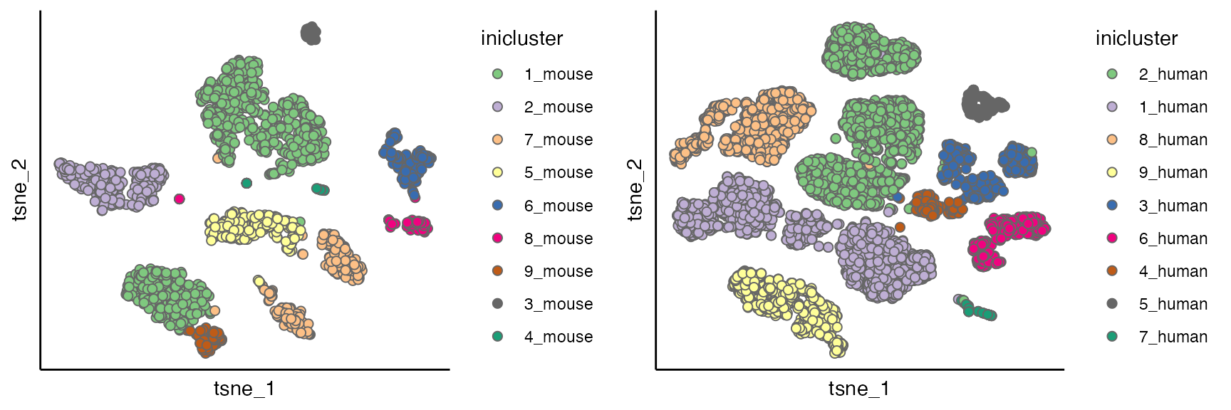
scatterPlot(seu_list[[2]], "tsne", "Group")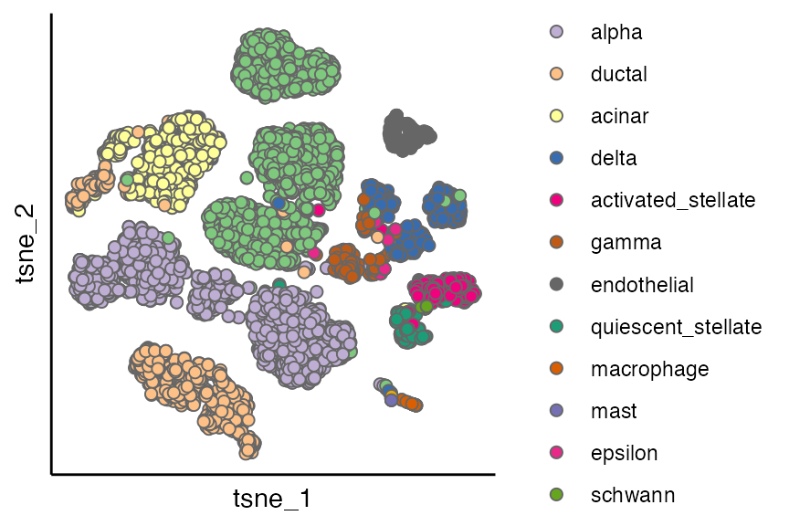
Calculate of IDER similarity matrix
res <- unlist(lapply(seu_list, function(x) return(x$inicluster)))
res_names <- unlist(lapply(seu_list, function(x) return(colnames(x))))
seu@meta.data$initial_cluster <- res[match(colnames(seu), res_names)]

ider <- getIDEr(seu,
                group.by.var = "initial_cluster",
                batch.by.var = "Batch",
                downsampling.size = 35,
                use.parallel = FALSE, verbose = FALSE)
net <- plotNetwork(seu, ider, colour.by = "Group" , vertex.size = 0.6, weight.factor = 5)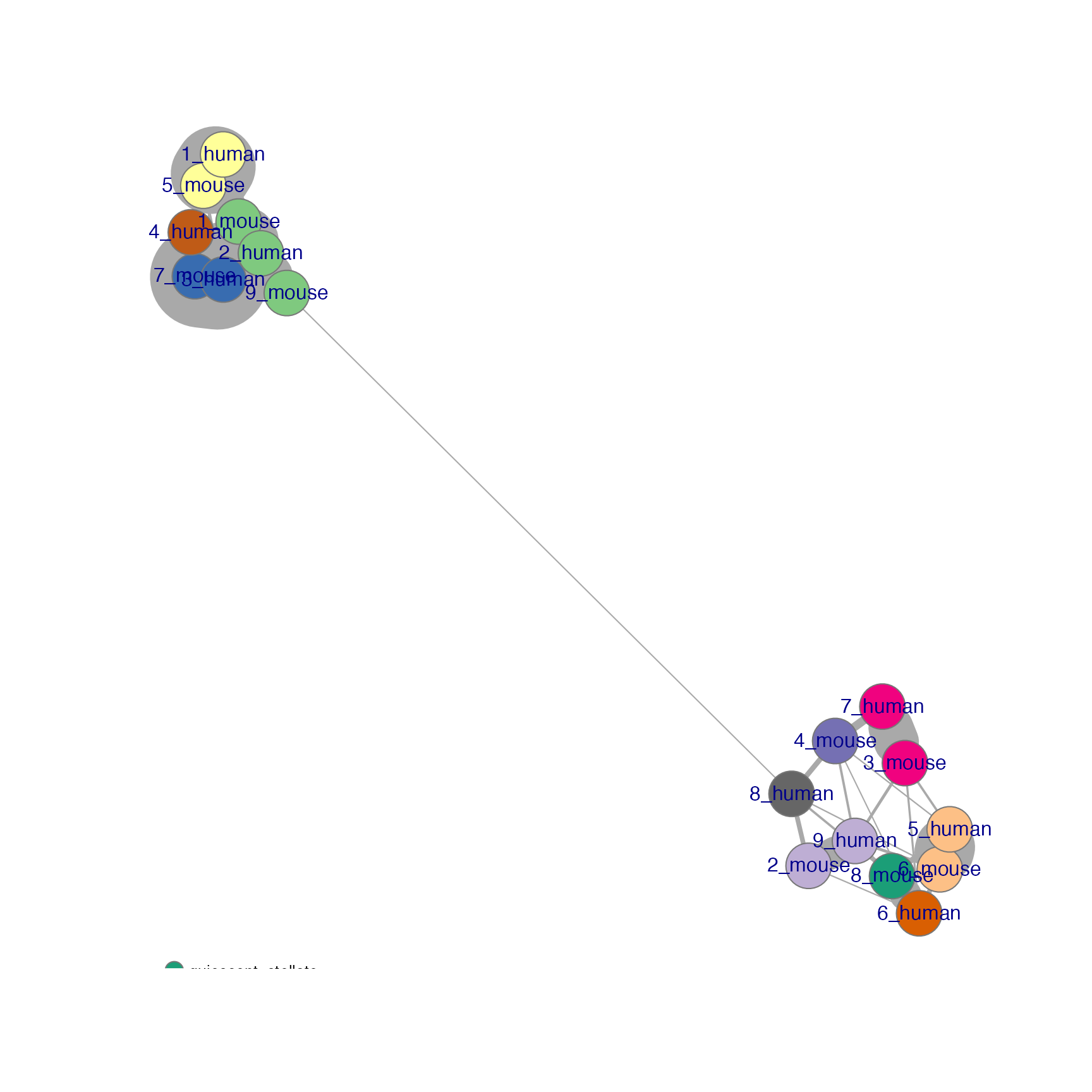
hc <- hclust(as.dist(1-(ider[[1]] + t(ider[[1]])))/2)
plot(as.dendrogram(hc)) #, horiz = TRUE
Perform final Clustering
seu <- finalClustering(seu, ider, cutree.h = 0.35) # final clustering
seu <- NormalizeData(seu, verbose = FALSE)
seu <- FindVariableFeatures(seu, selection.method = "vst",
                            nfeatures = 2000, verbose = FALSE)
seu <- ScaleData(seu, verbose = FALSE)
seu <- RunPCA(seu, npcs = 20, verbose = FALSE)
seu <- RunTSNE(seu, reduction = "pca", dims = 1:12)
plot_list <- list()
plot_list[[1]] <- scatterPlot(seu, "tsne", colour.by = "CIDER_cluster", title = "asCIDER clustering results")
plot_list[[2]] <- scatterPlot(seu, "tsne", colour.by = "Group", title = "Ground truth of cell populations")
plot_grid(plotlist = plot_list, ncol = 2)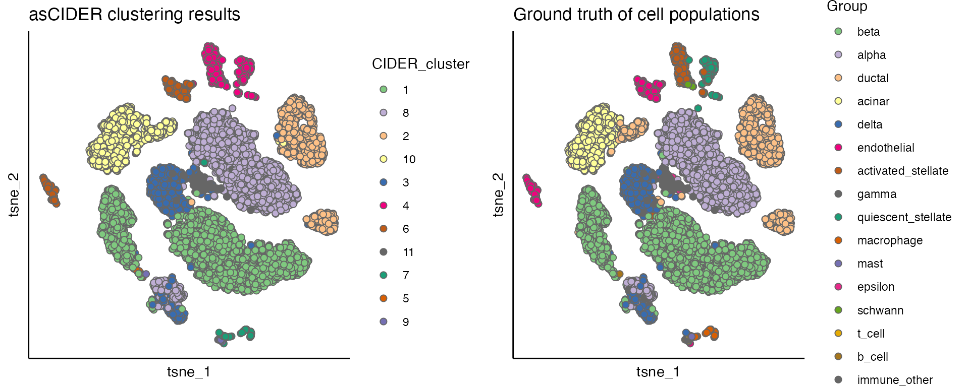
Reproducibility
sessionInfo()
#> R version 4.4.1 (2024-06-14)
#> Platform: x86_64-apple-darwin20
#> Running under: macOS Monterey 12.5.1
#>
#> Matrix products: default
#> BLAS:   /Library/Frameworks/R.framework/Versions/4.4-x86_64/Resources/lib/libRblas.0.dylib
#> LAPACK: /Library/Frameworks/R.framework/Versions/4.4-x86_64/Resources/lib/libRlapack.dylib;  LAPACK version 3.12.0
#>
#> locale:
#> [1] en_US.UTF-8/en_US.UTF-8/en_US.UTF-8/C/en_US.UTF-8/en_US.UTF-8
#>
#> time zone: Europe/London
#> tzcode source: internal
#>
#> attached base packages:
#> [1] parallel  stats     graphics  grDevices utils     datasets  methods
#> [8] base
#>
#> other attached packages:
#> [1] cowplot_1.1.3      Seurat_5.1.0       SeuratObject_5.0.2 sp_2.1-4
#> [5] CIDER_0.99.4
#>
#> loaded via a namespace (and not attached):
#>   [1] RColorBrewer_1.1-3     rstudioapi_0.16.0      jsonlite_1.8.8
#>   [4] magrittr_2.0.3         spatstat.utils_3.1-0   farver_2.1.2
#>   [7] rmarkdown_2.27         fs_1.6.4               ragg_1.3.2
#>  [10] vctrs_0.6.5            ROCR_1.0-11            spatstat.explore_3.3-2
#>  [13] htmltools_0.5.8.1      sass_0.4.9             sctransform_0.4.1
#>  [16] parallelly_1.38.0      KernSmooth_2.23-24     bslib_0.7.0
#>  [19] htmlwidgets_1.6.4      desc_1.4.3             ica_1.0-3
#>  [22] plyr_1.8.9             plotly_4.10.4          zoo_1.8-12
#>  [25] cachem_1.1.0           igraph_2.0.3           mime_0.12
#>  [28] lifecycle_1.0.4        iterators_1.0.14       pkgconfig_2.0.3
#>  [31] Matrix_1.7-0           R6_2.5.1               fastmap_1.2.0
#>  [34] fitdistrplus_1.2-1     future_1.34.0          shiny_1.9.1
#>  [37] digest_0.6.37          colorspace_2.1-1       patchwork_1.2.0
#>  [40] tensor_1.5             RSpectra_0.16-2        irlba_2.3.5.1
#>  [43] textshaping_0.4.0      labeling_0.4.3         progressr_0.14.0
#>  [46] fansi_1.0.6            spatstat.sparse_3.1-0  httr_1.4.7
#>  [49] polyclip_1.10-7        abind_1.4-5            compiler_4.4.1
#>  [52] withr_3.0.1            doParallel_1.0.17      viridis_0.6.5
#>  [55] fastDummies_1.7.4      highr_0.11             MASS_7.3-61
#>  [58] tools_4.4.1            lmtest_0.9-40          httpuv_1.6.15
#>  [61] future.apply_1.11.2    goftest_1.2-3          glue_1.7.0
#>  [64] dbscan_1.2.2           nlme_3.1-165           promises_1.3.0
#>  [67] grid_4.4.1             Rtsne_0.17             cluster_2.1.6
#>  [70] reshape2_1.4.4         generics_0.1.3         gtable_0.3.5
#>  [73] spatstat.data_3.1-2    tidyr_1.3.1            data.table_1.16.0
#>  [76] utf8_1.2.4             spatstat.geom_3.3-2    RcppAnnoy_0.0.22
#>  [79] ggrepel_0.9.5          RANN_2.6.2             foreach_1.5.2
#>  [82] pillar_1.9.0           stringr_1.5.1          limma_3.60.6
#>  [85] spam_2.10-0            RcppHNSW_0.6.0         later_1.3.2
#>  [88] splines_4.4.1          dplyr_1.1.4            lattice_0.22-6
#>  [91] survival_3.7-0         deldir_2.0-4           tidyselect_1.2.1
#>  [94] locfit_1.5-9.10        miniUI_0.1.1.1         pbapply_1.7-2
#>  [97] knitr_1.48             gridExtra_2.3          edgeR_4.2.2
#> [100] scattermore_1.2        xfun_0.46              statmod_1.5.0
#> [103] matrixStats_1.4.1      pheatmap_1.0.12        stringi_1.8.4
#> [106] lazyeval_0.2.2         yaml_2.3.10            evaluate_0.24.0
#> [109] codetools_0.2-20       kernlab_0.9-33         tibble_3.2.1
#> [112] cli_3.6.3              uwot_0.2.2             xtable_1.8-4
#> [115] reticulate_1.39.0      systemfonts_1.1.0      munsell_0.5.1
#> [118] jquerylib_0.1.4        Rcpp_1.0.13            globals_0.16.3
#> [121] spatstat.random_3.3-1  png_0.1-8              spatstat.univar_3.0-1
#> [124] pkgdown_2.1.0          ggplot2_3.5.1          dotCall64_1.1-1
#> [127] listenv_0.9.1          viridisLite_0.4.2      scales_1.3.0
#> [130] ggridges_0.5.6         leiden_0.4.3.1         purrr_1.0.2
#> [133] rlang_1.1.4
References
- Baron, M. et al. A Single-Cell Transcriptomic Map of the Human and Mouse Pancreas Reveals Inter- and Intra-cell Population Structure. Cell Syst 3, 346–360.e4 (2016).
- Satija R, et al. Spatial reconstruction of single-cell gene expression data. Nature Biotechnology 33, 495-502 (2015).
- The count matrix and sample information were downloaded from NCBI GEO accession GSE84133.